5 Modeling
5.1 SQL Native sampling
Use PostgreSQL TABLESAMPLE clause
- Use
build_sql()andremote_query()to combine a thedplyrcommand with a custom SQL statement
sql_sample <- dbGetQuery(con, build_sql(remote_query(table_flights), " TABLESAMPLE SYSTEM (0.1)"))- Preview the sample data
sql_sample## flightid year month dayofmonth dayofweek deptime crsdeptime arrtime
## 1 33574 2008 1 13 7 1503 1505 1635
## 2 33575 2008 1 13 7 806 805 939
## 3 33576 2008 1 13 7 1000 1005 1133
## 4 33577 2008 1 13 7 1259 1305 1428
## 5 33578 2008 1 13 7 1646 1645 1826
## 6 33579 2008 1 13 7 1949 1945 2126
## 7 33580 2008 1 13 7 710 710 933
## 8 33581 2008 1 13 7 1002 1005 1322
## 9 33582 2008 1 13 7 1356 1400 1705
## 10 33583 2008 1 13 7 2119 2100 31
## 11 33584 2008 1 13 7 709 710 1034
## 12 33585 2008 1 13 7 1909 1740 2227
## 13 33586 2008 1 13 7 1030 1030 1150
## 14 33587 2008 1 13 7 1423 1415 1539
## 15 33588 2008 1 13 7 2115 2040 2238
## 16 33589 2008 1 13 7 1903 1810 2031
## 17 33590 2008 1 13 7 1402 1405 1539
## 18 33591 2008 1 13 7 900 900 1035
## 19 33592 2008 1 13 7 1227 1230 1346
## 20 33593 2008 1 13 7 1932 1915 2107
## 21 33594 2008 1 13 7 1720 1645 1856
## 22 33595 2008 1 13 7 1608 1505 1915
## 23 33596 2008 1 13 7 1653 1650 2025
## 24 33597 2008 1 13 7 732 735 1123
## 25 33598 2008 1 13 7 1929 1935 2023
## 26 33599 2008 1 13 7 731 735 835
## 27 33600 2008 1 13 7 1151 1145 1245
## 28 33601 2008 1 13 7 706 705 819
## 29 33602 2008 1 13 7 1607 1610 1722
## 30 33603 2008 1 13 7 710 715 1017
## 31 33604 2008 1 13 7 939 940 1102
## 32 33698 2008 1 13 7 1046 1035 1151
## crsarrtime uniquecarrier flightnum tailnum actualelapsedtime
## 1 1640 WN 2817 N745SW 92
## 2 940 WN 3310 N337SW 93
## 3 1140 WN 3398 N455WN 93
## 4 1435 WN 3490 N308SA 89
## 5 1820 WN 3685 N727SW 100
## 6 2120 WN 3766 N718SW 97
## 7 1015 WN 110 N748SW 323
## 8 1330 WN 127 N428WN 200
## 9 1720 WN 396 N789SW 189
## 10 15 WN 1076 N292WN 192
## 11 1035 WN 1462 N492WN 205
## 12 2055 WN 2532 N252WN 198
## 13 1205 WN 892 N257WN 140
## 14 1550 WN 2113 N790SW 136
## 15 2215 WN 3221 N678AA 143
## 16 1945 WN 3413 N366SW 148
## 17 1535 WN 54 N522SW 97
## 18 1030 WN 1086 N636WN 95
## 19 1355 WN 1375 N636WN 79
## 20 2045 WN 2115 N636WN 95
## 21 1815 WN 2133 N506SW 96
## 22 1900 WN 3915 N227WN 307
## 23 2025 WN 300 N714CB 212
## 24 1105 WN 806 N217JC 231
## 25 2050 WN 217 N603SW 54
## 26 850 WN 420 N736SA 64
## 27 1300 WN 1357 N388SW 54
## 28 825 WN 1531 N348SW 73
## 29 1735 WN 3307 N715SW 75
## 30 1030 WN 1589 N276WN 127
## 31 1105 WN 226 N768SW 83
## 32 1150 WN 1591 N613SW 65
## crselapsedtime airtime arrdelay depdelay origin dest distance taxiin
## 1 95 79 -5 -2 MHT BWI 377 5
## 2 95 77 -1 1 MHT BWI 377 6
## 3 95 75 -7 -5 MHT BWI 377 4
## 4 90 79 -7 -6 MHT BWI 377 4
## 5 95 83 6 1 MHT BWI 377 3
## 6 95 85 6 4 MHT BWI 377 3
## 7 365 306 -42 0 MHT LAS 2356 7
## 8 205 180 -8 -3 MHT MCO 1142 7
## 9 200 179 -15 -4 MHT MCO 1142 4
## 10 195 176 16 19 MHT MCO 1142 6
## 11 205 186 -1 -1 MHT MCO 1142 6
## 12 195 182 92 89 MHT MCO 1142 4
## 13 155 124 -15 0 MHT MDW 838 5
## 14 155 123 -11 8 MHT MDW 838 6
## 15 155 129 23 35 MHT MDW 838 5
## 16 155 123 46 53 MHT MDW 838 8
## 17 90 76 4 -3 MHT PHL 290 14
## 18 90 74 5 0 MHT PHL 290 12
## 19 85 65 -9 -3 MHT PHL 290 7
## 20 90 74 22 17 MHT PHL 290 11
## 21 90 76 41 35 MHT PHL 290 6
## 22 355 293 15 63 MHT PHX 2279 5
## 23 215 195 0 3 MHT TPA 1204 5
## 24 210 213 18 -3 MHT TPA 1204 3
## 25 75 43 -27 -6 MSY BHM 321 3
## 26 75 42 -15 -4 MSY BHM 321 15
## 27 75 45 -15 6 MSY BHM 321 4
## 28 80 64 -6 1 MSY BNA 471 3
## 29 85 63 -13 -3 MSY BNA 471 6
## 30 135 115 -13 -5 MSY BWI 998 6
## 31 85 70 -3 -1 MSY DAL 437 5
## 32 75 56 1 11 OAK ONT 361 3
## taxiout cancelled cancellationcode diverted carrierdelay weatherdelay
## 1 8 0 <NA> 0 0 0
## 2 10 0 <NA> 0 0 0
## 3 14 0 <NA> 0 0 0
## 4 6 0 <NA> 0 0 0
## 5 14 0 <NA> 0 0 0
## 6 9 0 <NA> 0 0 0
## 7 10 0 <NA> 0 0 0
## 8 13 0 <NA> 0 0 0
## 9 6 0 <NA> 0 0 0
## 10 10 0 <NA> 0 3 0
## 11 13 0 <NA> 0 0 0
## 12 12 0 <NA> 0 0 0
## 13 11 0 <NA> 0 0 0
## 14 7 0 <NA> 0 0 0
## 15 9 0 <NA> 0 0 0
## 16 17 0 <NA> 0 0 0
## 17 7 0 <NA> 0 0 0
## 18 9 0 <NA> 0 0 0
## 19 7 0 <NA> 0 0 0
## 20 10 0 <NA> 0 2 0
## 21 14 0 <NA> 0 22 0
## 22 9 0 <NA> 0 0 0
## 23 12 0 <NA> 0 0 0
## 24 15 0 <NA> 0 0 0
## 25 8 0 <NA> 0 0 0
## 26 7 0 <NA> 0 0 0
## 27 5 0 <NA> 0 0 0
## 28 6 0 <NA> 0 0 0
## 29 6 0 <NA> 0 0 0
## 30 6 0 <NA> 0 0 0
## 31 8 0 <NA> 0 0 0
## 32 6 0 <NA> 0 0 0
## nasdelay securitydelay lateaircraftdelay score
## 1 0.0000000 0 0 NA
## 2 0.0000000 0 0 NA
## 3 0.0000000 0 0 NA
## 4 0.0000000 0 0 NA
## 5 0.0000000 0 0 NA
## 6 0.0000000 0 0 NA
## 7 0.0000000 0 0 NA
## 8 0.0000000 0 0 NA
## 9 0.0000000 0 0 NA
## 10 0.0000000 0 13 NA
## 11 0.0000000 0 0 NA
## 12 3.0000000 0 89 NA
## 13 0.0000000 0 0 NA
## 14 0.0000000 0 0 NA
## 15 0.0000000 0 23 NA
## 16 36.0000000 0 10 NA
## 17 0.0000000 0 0 NA
## 18 0.0000000 0 0 NA
## 19 0.0000000 0 0 NA
## 20 5.0000000 0 15 NA
## 21 6.0000000 0 13 NA
## 22 0.0000000 0 15 NA
## 23 0.0000000 0 0 NA
## 24 18.0000000 0 0 NA
## 25 0.0000000 0 0 NA
## 26 0.0000000 0 0 NA
## 27 0.0000000 0 0 NA
## 28 0.0000000 0 0 NA
## 29 0.0000000 0 0 NA
## 30 0.0000000 0 0 NA
## 31 0.0000000 0 0 NA
## 32 0.0000000 0 0 NA
## [ reached getOption("max.print") -- omitted 6534 rows ]- Test the efficacy of the sampling with a plot
dbplot_histogram(sql_sample, distance)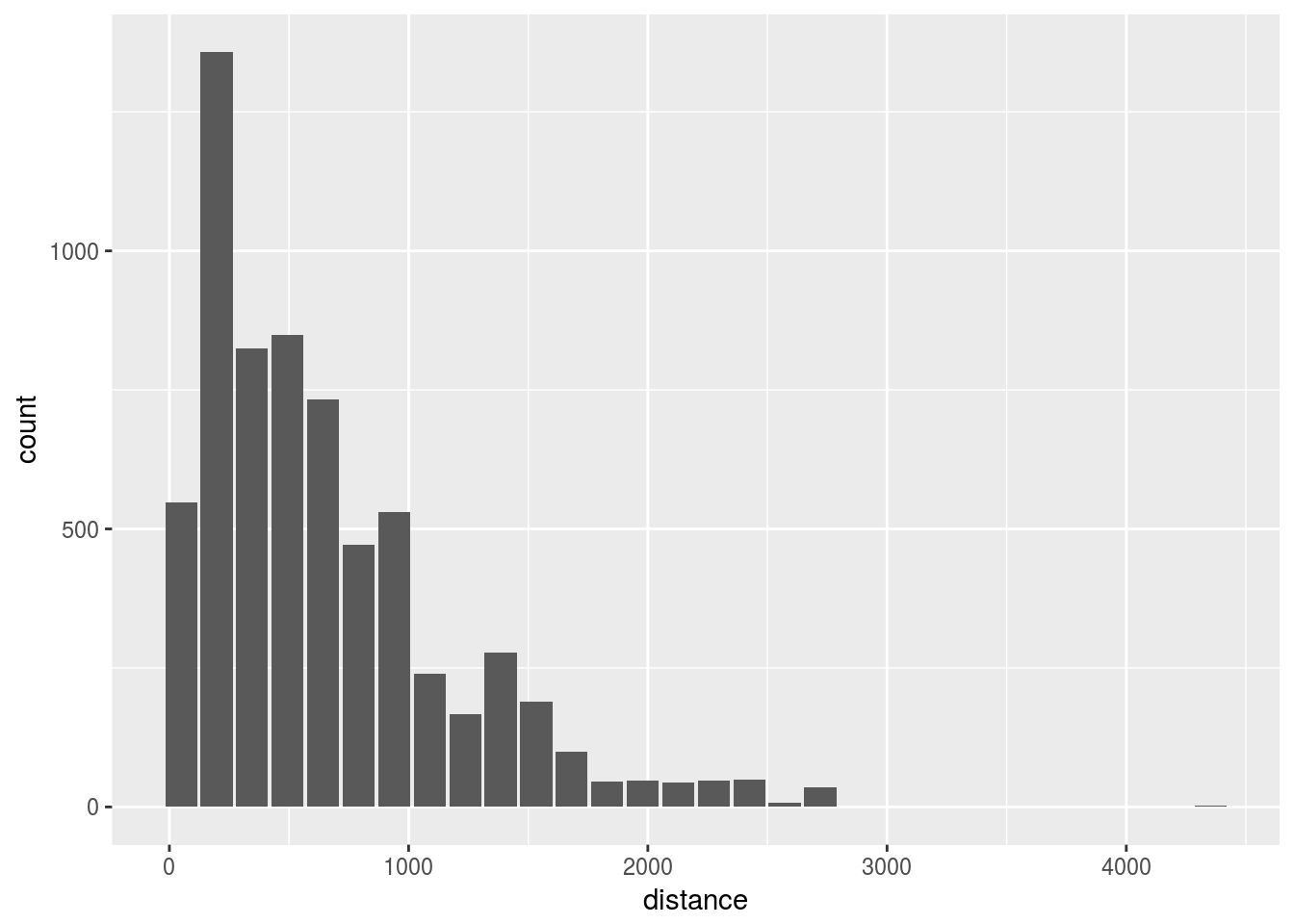
5.2 Sample with ID
Use a record’s unique ID to produce a sample
- Use
max()to get the upper limit for flightid
limit <- table_flights %>%
  summarise(
    max = max(flightid, na.rm = TRUE),
    min = min(flightid, na.rm = TRUE)
  ) %>%
collect()- Use
sampleto get 0.1% of IDs
sampling <- sample(
  limit$min:limit$max,
round((limit$max -limit$min) * 0.001))- Use
%in%to match the sample IDs in the flight table
id_sample <- table_flights %>%
  filter(flightid %in% sampling) %>%
  collect()
Verify sample with a histogram
dbplot_histogram(id_sample, distance)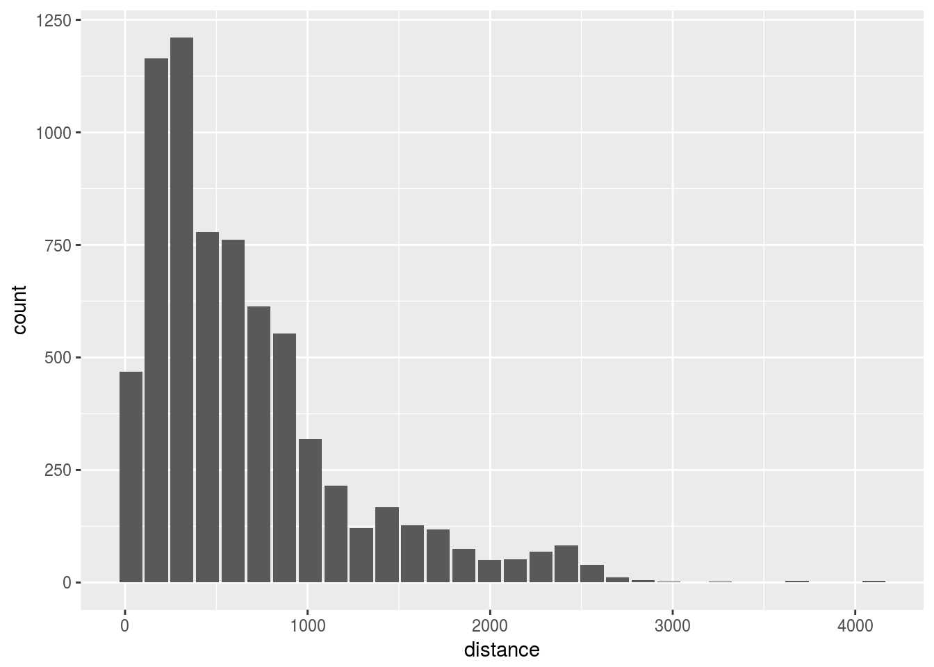
5.3 Sample manually
Use row_number(), sample() and map_df() to create a sample data set
- Create a filtered dataset for with 1 month of data
db_month <- table_flights %>%
filter(month == 1)- Get the row count
rows <- as.integer(pull(tally(db_month)))- Use
row_number()to create a new column to number each row
db_month <- db_month %>%
mutate(row = row_number()) - Create a random set of 600 numbers, limited by the number of rows
sampling <- sample(1:rows, 600)- Use
%in%to filter the matched sample row IDs with the random set
db_month <- db_month %>%
filter(row %in% sampling)- Verify number of rows
tally(db_month)## # Source: lazy query [?? x 1]
## # Database: postgres [rstudio_dev@localhost:/postgres]
## n
## <S3: integer64>
## 1 600- Create a function with the previous steps, but replacing the month number with an argument. Collect the data at the end
sample_segment <- function(x, size = 600) {
  db_month <- table_flights %>%
    filter(month == x)
  rows <- as.integer(pull(tally(db_month)))
  db_month <- db_month %>%
    mutate(row = row_number())
  sampling <- sample(1:rows, size)
  db_month %>%
    filter(row %in% sampling) %>%
    collect()
}- Test the function
head(sample_segment(3), 100)## # A tibble: 100 x 32
## flightid year month dayofmonth dayofweek deptime crsdeptime arrtime
## <int> <dbl> <dbl> <dbl> <dbl> <dbl> <dbl> <dbl>
## 1 1177397 2008 3.00 3.00 1.00 1255 1300 1757
## 2 1178163 2008 3.00 4.00 2.00 0 1100 0
## 3 1178843 2008 3.00 4.00 2.00 2014 2020 2313
## 4 1179181 2008 3.00 4.00 2.00 1234 1240 1538
## 5 1179383 2008 3.00 4.00 2.00 910 910 1611
## 6 1183508 2008 3.00 5.00 3.00 1503 1505 1843
## 7 1184320 2008 3.00 5.00 3.00 1501 1500 1624
## 8 1185900 2008 3.00 6.00 4.00 2044 1800 2138
## 9 1188586 2008 3.00 7.00 5.00 2105 1745 2317
## 10 1191354 2008 3.00 7.00 5.00 1740 1700 2345
## # ... with 90 more rows, and 24 more variables: crsarrtime <dbl>,
## # uniquecarrier <chr>, flightnum <dbl>, tailnum <chr>,
## # actualelapsedtime <dbl>, crselapsedtime <dbl>, airtime <dbl>,
## # arrdelay <dbl>, depdelay <dbl>, origin <chr>, dest <chr>,
## # distance <dbl>, taxiin <dbl>, taxiout <dbl>, cancelled <dbl>,
## # cancellationcode <chr>, diverted <dbl>, carrierdelay <dbl>,
## # weatherdelay <dbl>, nasdelay <dbl>, securitydelay <dbl>,
## # lateaircraftdelay <dbl>, score <int>, row <S3: integer64>- Use
map_df()to run the function for each month
strat_sample <- 1:12 %>%
map_df(~sample_segment(.x))- Verify sample with a histogram
dbplot_histogram(strat_sample, distance)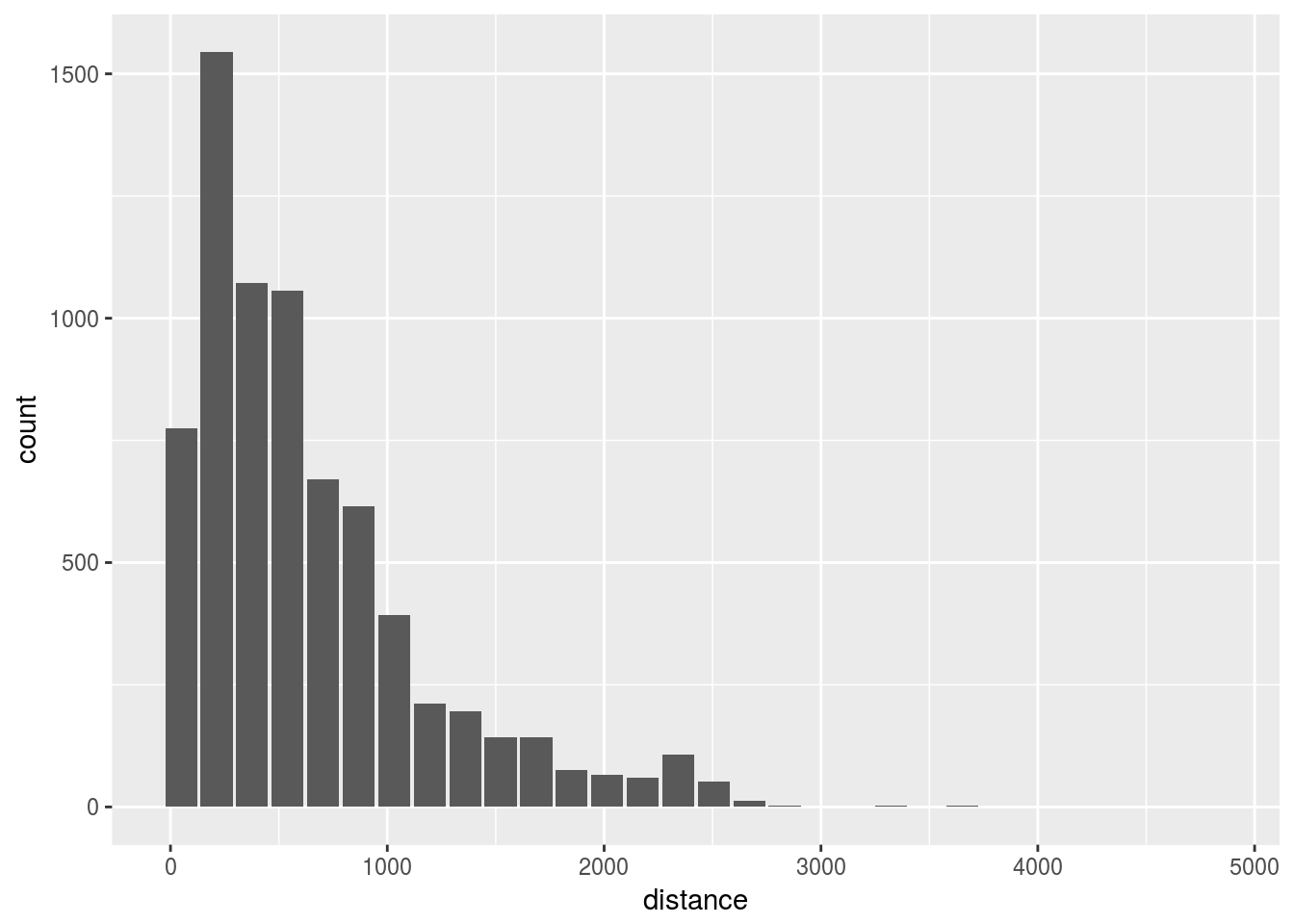
5.4 Create a model & test
- Prepare a model data set
model_data <- strat_sample %>%
    mutate(
    season = case_when(
      month >= 3 & month <= 5  ~ "Spring",
      month >= 6 & month <= 8  ~ "Summmer",
      month >= 9 & month <= 11 ~ "Fall",
      month == 12 | month <= 2  ~ "Winter"
    )
  ) %>%
select(arrdelay, season, depdelay) - Create a simple
lm()model
model_lm <- lm(arrdelay ~ . , data = model_data)
summary(model_lm)
##
## Call:
## lm(formula = arrdelay ~ ., data = model_data)
##
## Residuals:
## Min 1Q Median 3Q Max
## -319.63 -7.38 -1.31 5.46 153.40
##
## Coefficients:
## Estimate Std. Error t value Pr(>|t|)
## (Intercept) -3.555680 0.333985 -10.646 < 2e-16 ***
## seasonSpring 1.899032 0.471854 4.025 5.77e-05 ***
## seasonSummmer 2.164639 0.472263 4.584 4.65e-06 ***
## seasonWinter 2.574540 0.473742 5.434 5.68e-08 ***
## depdelay 0.986506 0.004536 217.469 < 2e-16 ***
## ---
## Signif. codes: 0 '***' 0.001 '**' 0.01 '*' 0.05 '.' 0.1 ' ' 1
##
## Residual standard error: 14.14 on 7195 degrees of freedom
## Multiple R-squared: 0.8698, Adjusted R-squared: 0.8698
## F-statistic: 1.202e+04 on 4 and 7195 DF, p-value: < 2.2e-16- Create a test data set by combining the sampling and model data set routines
test_sample <- 1:12 %>%
  map_df(~sample_segment(.x, 100)) %>%
    mutate(
    season = case_when(
      month >= 3 & month <= 5  ~ "Spring",
      month >= 6 & month <= 8  ~ "Summmer",
      month >= 9 & month <= 11 ~ "Fall",
      month == 12 | month <= 2  ~ "Winter"
    )
  ) %>%
select(arrdelay, season, depdelay) - Run a simple routine to check accuracy
test_sample %>%
  mutate(p = predict(model_lm, test_sample),
         over = abs(p - arrdelay) < 10) %>%
  group_by(over) %>%
  tally() %>%
  mutate(percent = round(n / sum(n), 2))
## # A tibble: 2 x 3
## over n percent
## <lgl> <int> <dbl>
## 1 F 398 0.330
## 2 T 802 0.6705.5 Score inside database
Learn about tidypredict to run predictions inside the database
- Load the library, and see the results of passing the model as an argument to
tidypredict_fit()
library(tidypredict)

tidypredict_fit(model_lm)
## ((((-3.55567950836314) + ((ifelse((season) == ("Spring"), 1,
## 0)) * (1.89903163366937))) + ((ifelse((season) == ("Summmer"),
## 1, 0)) * (2.16463859693503))) + ((ifelse((season) == ("Winter"),
## 1, 0)) * (2.57453965992478))) + ((depdelay) * (0.98650585644528))- Use
tidypredict_sql()to see the resulting SQL statement
tidypredict_sql(model_lm, con)## <SQL> ((((-3.55567950836314) + ((CASE WHEN (("season") = ('Spring')) THEN (1.0) WHEN NOT(("season") = ('Spring')) THEN (0.0) END) * (1.89903163366937))) + ((CASE WHEN (("season") = ('Summmer')) THEN (1.0) WHEN NOT(("season") = ('Summmer')) THEN (0.0) END) * (2.16463859693503))) + ((CASE WHEN (("season") = ('Winter')) THEN (1.0) WHEN NOT(("season") = ('Winter')) THEN (0.0) END) * (2.57453965992478))) + (("depdelay") * (0.98650585644528))- Run the prediction inside
dplyr
table_flights %>%
  filter(month == 2,
         dayofmonth == 1) %>%
    mutate(
    season = case_when(
      month >= 3 & month <= 5  ~ "Spring",
      month >= 6 & month <= 8  ~ "Summmer",
      month >= 9 & month <= 11 ~ "Fall",
      month == 12 | month <= 2  ~ "Winter"
    )
  ) %>%
  select( season, depdelay) %>%
  tidypredict_to_column(model_lm) %>%
  head()
## # Source: lazy query [?? x 3]
## # Database: postgres [rstudio_dev@localhost:/postgres]
## season depdelay fit
## <chr> <dbl> <dbl>
## 1 Winter 19.0 17.8
## 2 Winter 0 - 0.981
## 3 Winter - 5.00 - 5.91
## 4 Winter - 9.00 - 9.86
## 5 Winter - 6.00 - 6.90
## 6 Winter 50.0 48.3- View the SQL behind the
dplyrcommand
table_flights %>%
  filter(month == 2,
         dayofmonth == 1) %>%
    mutate(
    season = case_when(
      month >= 3 & month <= 5  ~ "Spring",
      month >= 6 & month <= 8  ~ "Summmer",
      month >= 9 & month <= 11 ~ "Fall",
      month == 12 | month <= 2  ~ "Winter"
    )
  ) %>%
  select( season, depdelay) %>%
  tidypredict_to_column(model_lm) %>%
  remote_query()
## <SQL> SELECT "season", "depdelay", ((((-3.55567950836314) + ((CASE WHEN (("season") = ('Spring')) THEN (1.0) WHEN NOT(("season") = ('Spring')) THEN (0.0) END) * (1.89903163366937))) + ((CASE WHEN (("season") = ('Summmer')) THEN (1.0) WHEN NOT(("season") = ('Summmer')) THEN (0.0) END) * (2.16463859693503))) + ((CASE WHEN (("season") = ('Winter')) THEN (1.0) WHEN NOT(("season") = ('Winter')) THEN (0.0) END) * (2.57453965992478))) + (("depdelay") * (0.98650585644528)) AS "fit"
## FROM (SELECT "season", "depdelay"
## FROM (SELECT "flightid", "year", "month", "dayofmonth", "dayofweek", "deptime", "crsdeptime", "arrtime", "crsarrtime", "uniquecarrier", "flightnum", "tailnum", "actualelapsedtime", "crselapsedtime", "airtime", "arrdelay", "depdelay", "origin", "dest", "distance", "taxiin", "taxiout", "cancelled", "cancellationcode", "diverted", "carrierdelay", "weatherdelay", "nasdelay", "securitydelay", "lateaircraftdelay", "score", CASE
## WHEN ("month" >= 3.0 AND "month" <= 5.0) THEN ('Spring')
## WHEN ("month" >= 6.0 AND "month" <= 8.0) THEN ('Summmer')
## WHEN ("month" >= 9.0 AND "month" <= 11.0) THEN ('Fall')
## WHEN ("month" = 12.0 OR "month" <= 2.0) THEN ('Winter')
## END AS "season"
## FROM (SELECT *
## FROM datawarehouse.flight
## WHERE (("month" = 2.0) AND ("dayofmonth" = 1.0))) "rdmsrldtdf") "xsktnwfckl") "pifkbjpiqq"- Compare predictions to ensure results are within range
test <- tidypredict_test(model_lm)
test
## tidypredict test results
## Difference threshold: 1e-12
##
## All results are within the difference threshold- View the records that exceeded the threshold
test$raw_results %>%
  filter(fit_threshold)
## [1] rowid fit fit_te fit_diff fit_threshold
## <0 rows> (or 0-length row.names)5.6 Parsed model
Quick review of the model parser
- Use the
parse_model()function to see howtidypredictinterprets the model
pm <- parse_model(model_lm)
pm
## # A tibble: 10 x 11
## labels estimate type field_1 field_2 qr_1 qr_2 qr_3
## <chr> <dbl> <chr> <chr> <chr> <dbl> <dbl> <dbl>
## 1 (Intercep… - 3.56 term <NA> <NA> - 0.0118 - 0.00680 - 0.00962
## 2 seasonSpr… 1.90 term <NA> Spring 0 0.0272 0.00962
## 3 seasonSum… 2.16 term <NA> Summmer 0 0 0.0289
## 4 seasonWin… 2.57 term <NA> Winter 0 0 0
## 5 depdelay 0.987 term {{:}} <NA> 0 0 0
## 6 labels 0 varia… depdel… season NA NA NA
## 7 model NA varia… <NA> <NA> NA NA NA
## 8 version NA varia… <NA> <NA> NA NA NA
## 9 residual NA varia… <NA> <NA> NA NA NA
## 10 sigma2 NA varia… <NA> <NA> NA NA NA
## # ... with 3 more variables: qr_4 <dbl>, qr_5 <dbl>, vals <chr>- Verify that the resulting table can be used to get the fit formula
tidypredict_fit(pm)## ((((-3.55567950836314) + ((ifelse((season) == ("Spring"), 1,
## 0)) * (1.89903163366937))) + ((ifelse((season) == ("Summmer"),
## 1, 0)) * (2.16463859693503))) + ((ifelse((season) == ("Winter"),
## 1, 0)) * (2.57453965992478))) + ((depdelay) * (0.98650585644528))- Save the parsed model for later use
library(readr)
write_csv(pm, "parsedmodel.csv")- Disconnect from the database
dbDisconnect(con)